Another Post regarding recessions and TAA

I previously posted regarding the connection between returns of a TAA portfolio and when a recession occurs. This follow up with discuss the methodology and results from adjusting an investment strategy based on a quantitative estimate of the future probability of a recession.

The TAA models are good at reducing risk, but to increase return to something comparable to an equity index it seems silly to use the same amount of margin at all times. The post above gives evidence that lowering the amount of leverage in times when there is a prediction of a U.S. recession will increase the Sharpe ratio relative to a similarly levered model.

To incorporate this insight into the TAA model, as I used the same probit modeled I discussed in the first post I made regarding probit models. To use this model in an investing environment, I used a warm-up period of 200 months and then estimated the model each month to get a probability of a recession 12 months out. Since the NBER doesn't have dates for recessions in the past two years (I guestimated), I stopped the model 24 months prior to the end of February and used the coefficients as of that date with the data available to get the remaining predictions. Using this data I created two possible ways to scale in and out for leverage. I looked back four months for predictions in both cases. I did this for three reasons: the data constantly gets revised, I'm not sure always what is available on any given date and I want to be safe, and the lag time seems optimal (12 keeps you unlevered during the rebound, 1 is too sensitive, 6 works just as well, but I wanted to keep it shorter). So looking back four months, the first method will lever the portfolio when the estimated probability is greater than 50% and not lever the portfolio below that. The second method is similar except it provides three baskets levering a full amount, 50% of the full amount and none at all.

The results for the first and second method are comparable, but the second method slightly underperforms the first on a Sharpe ratio basis (the return is lower and the standard deviation is lower, but not by enough to offset the return). It's possible to fiddle with the parameters to improve the results, I'd rather just ignore it for the simplicity of the first model. The chart below gives the portfolio statistics for the first model with 0 leverage (and no probit data), 50% leverage, and 100% leverage. The first two columns are the base 0% and 50% and the probit columns represent the model with dynamic leverage ratios. Similar to before, I report the evenly weighted portfolios and the risk parity portfolios.

The results confirm my original intuition(!) and then the models even outperform what I had suspected would happen. Essentially the model reduces your leverage heading into a recession and then quickly puts it back on. Surprisingly, comparing these returns with the raw results from the last post on TAA and probits, shows an even better return for this method using the model than reducing leverage when a recession happened. I do use domestic equity volatility as a factor in the model which could help the investor get out when volatility increases (it is a small component compared to interest rates and money supply data though). Anyway, the results show an increase of the 50% leveraged portfolio's Sharpe ratio by almost .1 by reducing standard deviation substantially and keeping the returns constant. The 50% portfolio, previously with a horrible Sharpe ratio relative to the 0%, now is roughly comparable (with equal and risk parity weights). With 100% leverage, the risk parity probit model now has a Sharpe ratio equivalent to the equal weight 0% and 50% equal weight portfolios (but with more return and risk). However, the 100% leveraged probit models dramatically outperform their cousins without the probit model. Again, this is due to substantially reducing volatility by reducing leverage in periods leading up to recessions.

Given the success of the probit model in reducing volatility and keeping returns high, I now plan to investigate leverage as a function of the volatility of each asset class (individually). I'm guessing there would be similar results, but without some of the messier complications of using the probit model (not sure when data is released and it's relatively intensive computationally). Assuming I can find daily data from the site I got the monthly data, it shouldn't be that much of a problem and I can just use the percentage of large up and down days in a quarter as a proxy for volatility of each asset class.

A Preliminary Post regarding recessions and TAA

I was hoping to incorporate my recession model into decisions about margin into the TAA model previously blogged about (here and here), but things got away from me. The model is in Matlab and output recession predictions based on the information available at the time which was the big challenge so it really won’t be that much work beyond that. Hopefully, I can post that information tomorrow, but today I wanted to just give a brief update on the returns of the even Asset Allocation (20% in US stocks, Foreign Stocks, commodities, bonds, and REITs) vs. the returns of the Tactical version during times of recession.

I regressed the returns of the TAA strategy and the returns of the 50% levered TAA strategy against the returns on the comparable AA strategy (unlevered or levered) and a binary variable equal to 0 if the economy is not in a recession and 1 if the economy is in a recession. I’m saving the reader the time of reviewing the results, but the AA returns are highly significant (as expected) and the coefficient on the binary variable is not significant at the 5% level, but is at the 10% level for both levered and unlevered. I’m willing to concede that the effect on the adjusted R squared of the binary variable is very small, but the important thing is the sign of the coefficient and not necessarily how much of the variation is explained.

In both versions, the coefficient on the AA variable is roughly .61, but the intercept and the coefficient on the binary variable are roughly .003 and .004 in the unlevered and levered versions, respectively. These numbers are based on monthly returns, the annualized numbers are roughly 3.5% and 5%. For those without a statistical background, that means that in CAPM terms, the alpha is positive and larger for the levered version and, more importantly, both models outperform the passive strategies during recessions by a statistically and economically significant margin.

I tried to alternative strategies that could be considered a middle road. I developed two new returns variables based on the TAA data, the first was the unlevered TAA returns when there was no recession and levered otherwise and vice versa for the second. Looking at the regression results for these two gives evidence of being able to target which coefficient will be higher. Avoiding leverage in a recession increases the intercept to .004 and keeps the other coefficient flat, but avoiding leverage unless in a recession keeps the intercept, but the coefficient on the binary variable goes up to .004. Which is more important and why does it matter?

Ultimately looking at the return characteristics (below) yields the answer. As expected, the TAA model has the best Sharpe ratio; however, by avoiding margin during times of recession, you can increase the Sharpe ratio relative to a similarly leveraged portfolio. I haven’t been sure if I calculate the margin returns properly. Intuitively you would think that it would be double the returns minus the cost of debt, but with the TAA model you only margin the positions that you are in since the cost of margin is greater than the cost of cash. Furthermore, there are historical periods where the broker’s call rate gets so insanely large that it wouldn’t make sense to use margin, but this model, at present times, still uses it.

To conclude, by using a model that can predict recessions (which I conveniently have), you can improve the Sharpe ratio of leveraged portfolios. One possible note is that my model works to predict a recession within the next 12 months. It begins to show indications several months prior to a recession with plenty of time to take some off. Unfortunately this also means that there are several different ways to test it. Finally, I suspect that controlling the use of margin based on expected returns of the portfolio will also prove to enhance returns.

Probit Models and Crisis

In a typical linear regression model, you would regress something like yt=b1+b2*xt+e (t is a subscript and e represents error). Many are aware of this concept. However, there are many assumptions that must be made in order to get the math to be correct in OLS. Due to these assumptions, such as constant variance and normality of residual errors, if you yt dependent variable consists of only 0 and 1 or is truncated by any other means, then you will have misspecified your model. Given some series xt and b1 and b2, it is possible to predict yt much larger than 1 or smaller than 0. Two questions arise, how do you correct for this and why does it matter?

The main method to correct for truncated variables is to use a probit or logit model. The concept behind probit and logit is essentially the same except that they use different means to make a correction. In a probit model, instead of estimating the equation above that is yt=b1+b2*xt, you would estimate yt=phi(c1+c2*xt) where phi is the cumulative normal distribution. Since the cumulative normal distribution is bound by 0 to 1, then any values that are chosen within the parentheses can only predict values of y between 0 and 1. The logit model is similar, but instead of weighing by the normal distribution, it uses a calculation based on e^x and natural logs.
And why does it matter? These models are meant to estimate the likelihood that events will take place or not (this is the 0 and 1). The benefit of the normal distribution is that you're actually estimating the probability that a particular event will take place given your independent variables. I can think of two uses of an econometric model, to explain the past and explain the future. Econometric models have their uses in the former, but many times drastically fail in the latter. It is possible that the models are misspecified or that fundamental relationships are not merely absent, but are immeasurable. Furthermore, the models may not be stable which can cause forecasting errors to be too large to be useful. However, I find probit models to be a useful alternative to typical forecasting when events can be categorized as binary.

My primary use of the probit models follows in the footsteps of Wright (06-07) by examining the NBER dataset of business cycle dates. Wright uses a binary variable equal to 1 if there would be a recession within the next x months and 0 otherwise. Originally in my research, I attempted multiple lags forward such as 6,12,16 months ahead, but I eventually focused in on the 12 month as a base to compare alternative models. I continued to investigate additional variables and have settled on a fair group of variables that outperforms Wright's variables while maintaining and important economic significance of each. I continued to use the Fed Funds and the spread of long-term treasuries over the effective fed funds rate. I added the spread of the Fed Funds relative to BAA corporate securities adding a factor that includes the markets tolerance for risky debt (TED isn't as strong as this one) as well as measure of volatility of the S&P500 (% of days in last quarter with a change greater than or less than 1.25%). Finally, I added the most important component which is the money supply measure. Following Paul Kasriel (originally testing Mish's MPrime), I use the long-term change in real monetary base (bank reserves +currency divided by CPI). Positive values of this indicator represent expansionary monetary policy while negative shows that the Fed is tightening the money supply. As Mr. Kasriel notes, this normally happens to curb an expansion and combined with an inverted yield curve represents a particularly powerful indicator of a recession.

Over the 40 years tested (had to exclude the recent ones since no NBER dating exists for the current financial crisis), these variables in a probit model correctly classify 91% of months as whether they are in a recession or not (defined by above 50%). It's recent track record is that the estimated probability of a recession in the next 12 months briefly went above 75% back in 2006 and then came up above 75% again in June of 2007. Nevertheless, I would use a figure above 50% to definitely eliminate any leverage in U.S. equities and possibly cut down size (and an increasing trend in general as a sign to cut down) , above 75% means "Sell Mortimer!" The high values in June 2007 were driven by real monetary base values that were historically low. In previous episodes it barely crosses into negative values, but it has stayed essentially flat since then.

I have been mulling over the implications of this model for several months. In particular, the model estimates the probability of a recession, but the probabilities increase during all financial crises. For example, in times of large volatility or greater credit risk (flight to safety) or future rate cuts, this number increases. I wondered whether it would be appropriate to test times of financial crisis and recession using this model (how to measure, but at least my false positive in 1998 would go away) . However, even if this financial crisis is not called a recession, I wouldn't say this model failed because it was predicting one. A serious financial crisis occurred and a significant stock market correction. Using this model to avoid those situations is much more important than the classification.

Thoughts on inflation

"Inflation is always and everywhere a monetary phenomenon." - tons of Economists

With equity markets dropping today and a record increase in Non-Farm Payrolls, I thought I would begin a discussion on the determinants of inflation and what it means when there is a recession and what it means for asset allocation.

Inflation really only makes sense when you refer to it as the debasement of a currency. Simply put, governments and central banks print too much money in order to reduce interest rates. Consumers borrow more and drive up the prices of existing goods. The market process contribution to this reasoning is that the changes do not happen instantaneously, but happen over time. This causes real dislocations in the economy which helps bring about the business cycle.

Market process theorists, monetarists, and others have used money supply data to guide them to central banking policies towards the creation of money. I really don't have the answers as to which one to use or not not use. For example, I don't know whether Travelers Checks or TAF should be included. I prefer to stick with monetary base adjusted for inflation (so that I can compare it between periods). Monetary base is cash plus reserves, it's simple and easy to use. The long-term change in this statistic is a good indicator to reflect monetary policy. When it is increasing, it means the Fed is creating money faster than the money is being debased.

This graph is courtesy of Paul Kasriel. Periods of increasing real monetary base are associated with boom times and periods of decreasing RMB typically coincide with recessions or other economic crises (not necessarily a recession defined by NBER). Currently facing a period of declining RMB, we could have expected one or the other. The question to ask is, what now?

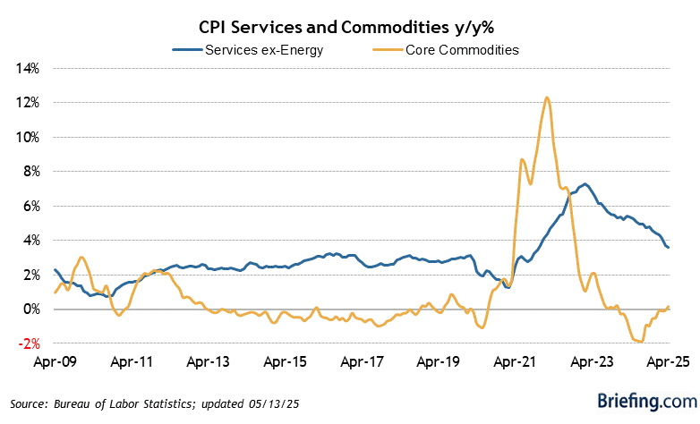
To understand the current inflation, it should be clear that agriculture and energy prices are a large component in headline CPI. For example, the energy CPI index was .7% in January compared to .3% for the core number. Looking at the CPI chart below, core commodities, however, are actually relatively flat compared to the last boom. Core commodities (excludes food and energy commodities) also dropped significantly during the last recession as core commodities do. The reason is that as economic and industrial activity slows, metals such as zinc, copper, and aluminum are in less demand. If there is to be a recession, or any further slowing of economic activity, these core commodities will likely enter a bear market over the course of the slowdown.

Several market commentators are still worried about the possibility of inflation despite the fact that RMB is most decreasing. This is mostly due to a long-run bull run in commodities driven by agriculture and energy prices and a weaker dollar. Indeed, if we are entering a recession, industrial minerals should be beat down further than they are.

Above are the graphs for the past two years worth of DBA and DBB (the agricultural and base minerals etfs, respectively). DBA (and GLD and USO) have all been on a run lately. Some of this run is certainly based on fundamental factors (ethanol, the collapse of the financial markets, and market's determined belief in peak oil). However, I would caution anyone looking to put on new positions in these commodity classes to hedge your risk by shorting a value of DBB equal to the whole value of those positions. If the market thinks inflation will be coming down, industrial minerals will decline faster than the others since it fundamentally should do that. The spread will certainly widen though it might make sense to wait to put on the long side of the spread until there is a pullback or a naked position on the short side until the recent trend shows signs of ending. You don't have to think that inflation is going to decrease (which it usually does in recessions, but not always), but just that industrial minerals will decrease more than the rest of commodities.