I added in the combined the j/k momentum model and the TAA model for the commodity and currency strategies I described yesterday(before it was only TAA, but I know follow the guidelines described in this post). The results confirmed the reasoning in yesterday's post. Commodities historically (tested since 83) do not have a very powerful momentum strategy. However, the j/k strategy with countries and the TAA model combined outperforms using the TAA model individually on each country. However, the TAA model generates very few signals and would be better for a longer-term investor. The j/k model (with j=4, k=2, and investing in the top 25%) with TAA overlay has a CAGR/Stdev of 2.18 (CAGR: 9.5%) compared to .99 (CAGR: 12.4%) for the EAFE TAA strategy. The EAFE without currencies in the TAA has a Sharpe of about 1 and 1.14 with them. Those increase to 1.07 and 1.23 (1.04 and 1.19 for yesterday's). However, regressing the new excess returns on the individual TAA excess returns does not generate significant alpha (annualized 26 bps), but the Beta is only .81. Unlike yesterday's strategy (ex-currencies), this strategy does have a significant alpha (at 10%) of 50 basis points relative to the original TAA strategy with a Beta of .78 (it improves to significant at 5% with 55 basis points with the currencies relative to TAA with currencies compared to 30 bps for the strategy yesterday).
* 50% decreases the Sharpe of the foreign strategy by themselves, but increases the Sharpe of the OVERALL strategy, I just wanted to be consistent with previous posts
addendum: I should note that the returns to this strategy are over a long period of time, particularly since the currency strategy benefits from high interest rates. The Sharpe ratios come down significantly over the past ten years compared to the past thirty years. Since the strategy has maintained a more constant growth path (ie not the early/mid 80s), the country strategy improves the Sharpe from .83 to .96 for the TAA strategy (individual country TAA is .93). However, the inclusion of the currency strategy has a smaller effect (I don't take into account the declining value of the dollar on any assets besides currencies, so this could be understated) increasing the Sharpe ratio by .04-.05. It seems that compared to the 50% momentum strategy over the past ten years, the EAFE has outperformed historically so that the momentum strategy is relatively constant, but the EAFE outperforms. (.4 10 year Sharpe vs. .1 30 year) in the past few years. I'm not sure how long the EAFE will continue to outperform, but I would prefer the less volatile Sharpe ratio. Right now my thinking is that after taking into account the depreciation of all of these assets in dollar terms, the best cash strategy would be the currency strategy, but I'm not sure yet.
Showing posts with label commodities. Show all posts
Showing posts with label commodities. Show all posts
Wednesday, April 16, 2008


Tuesday, April 15, 2008
Commodities and Foreign Countries
Continuing on with my theme of finding ways to improve the TAA model (here, here, and here), I thought I would do some more research into a longer examination of a timing strategy, but breaking apart an index into its component parts. I don't use the momentum strategy described in my Component TAA, Part II post (noted above), but just the normal timing model after breaking apart the EAFE and GSCI into their components. The strategy is to go long the components above the 10 month SMA and be in cash otherwise, just like Mr. Faber's TAA strategy.
I'll start with the GSCI. I used data available from the Global Financial Database on Commodities futures since 1983 (except Natty Gas which is since 1990). Unfortunately, they didn't have all of the energy contracts and were missing a few of the other contracts. I kept each commodity subgroup (livestock, ag, energy, ind. metals, precious metals) the same weight and scaled up the components. I confirmed that this index has about a 94% correlation with the GSCI. I was a little disappointed with this figure (preferring higher than 97.5%), but I will make due with what I have. I tested just performing the timing on the sectors (since 91) and on the individual components (since 83). One thing is very clear, the GSCI is dominated by energy you cannot compare an equally weighted TAA strategy with the market-weighted portfolio in GSCI. If you compare the strategies, use weights close to GSCI.
With sectors and a buy and hold strategy, my returns are initially different than the GSCI, so I don't expect the best comparison for the timing, but with 94% correlation, I would expect similar trends. However, I found that the return/sd ratio increased for the GSCI strategy, but not the component strategy. Variance decreased, but returns decreased as well and the effect was not economically significant. On the other hand, the returns to the GSCI strategy are enhanced considerably. The returns and correlations are roughly the same if you break it down into all of the contracts weighted by what is in GSCI. I wouldn't be surprised if some of this result is due to the fact that many of these commodities contracts show considerable seasonal variation that cannot be reduced easily by using the 200 day MA the way that an equity indices returns are improved (they lack the seasonal variations) and that the aggregate figure trends better. A more complex strategy, such as taking advantage of contango or backwardation, might be more appropriate for the components of the GSCI. There are other indices that I could use to test this method since I didn't have all the contracts (I will use the CRB indices except energy which I will have to recreate).
Countries, on the other hand, do trend well and the timing strategy works very well on them. I used total return data and replicated the EAFE index since 1994 with a 99% correlation. Before that time period, I replaced the FTSE-100 with the All-Shares index and some other total return indices are used that don't have futures contracts for them.
(begin digression: I had to use alternative indices for some countries that didn't have total return indices for the whole period, however, the question is how the strategy improves on this Buy and Hold strategy and not necessarily on the EAFE. If it improves returns over a long period of time, you could reasonably assume that it would continue to outperform in the future with futures contracts available and that the returns that you have are highly correlated with what you would have had with futures contracts. The returns are probably slightly better since the indices used are all-share instead of focused, but you would also expect the variance to be higher, it is equivalent to using the Wilshire 5000 instead of S&P500: end digression).
I also didn't use all of the indices in the EAFE since some of them have very small weights and the countries don't have actively traded futures. The top 12 or so are good enough. In general the equal weighted strategy outperforms the EAFE weights (due to the 25% weight on Japan). The difference isn't large enough to concern ourselves about over the long-term (1.26 CAGR/STD vs. 1.25). Over the long-term, the buy and hold returns were different between the EAFE and weighing the individual components (since there are times when I don't have France or Singapore's total return indices), but again the comparison I want to make is between the trends and not the absolute levels. From 1970 to February of this year, the Buy and Hold for the EAFE had a CAGR/std ratio of .715 (CAGR=11.7%) and the component strategy was .82 (CAGR=13.1%). Overlaying the timing strategy increased the Sharpe ratio on the EAFE to .99 (CAGR=12.4%) and the component to 1.25 while increasing the return to 13.6%. Since 1988 (when I have data on France), the spread between the strategies has stayed strong although overall returns aren't as strong. The Buy and Hold on EAFE went from .43 to .64 and with the component strategy it went from .62 to .95.
The 6% Sharpe ratio of the original TAA strategy was about 1.0 (12.4% CAGR) since April of 1980 and 1.14 (12.3% CAGR) with a currencies strategy. Replacing the EAFE increases the Sharpe to roughly 1.04 (12.5% CAGR) in the original and 1.18 (12.4% CAGR). The excess returns show an insignificant alpha over the original TAA strategy, but with the currency strategy included there is a significant alpha of 30 bps which reduces to about 25 bps when currencies have a 3x weight (Sharpe of 1.31 vs. 1.27 originally).
Also note that this is a timing model just like the one before. There isn't the excessive trading costs of a momentum strategy. You would be in each country about 60-75% of the time and frequently for years at a time. Someone with a large account could use this strategy to help reduce risk while keeping returns constant (meaning more leverage could be used).
I'll start with the GSCI. I used data available from the Global Financial Database on Commodities futures since 1983 (except Natty Gas which is since 1990). Unfortunately, they didn't have all of the energy contracts and were missing a few of the other contracts. I kept each commodity subgroup (livestock, ag, energy, ind. metals, precious metals) the same weight and scaled up the components. I confirmed that this index has about a 94% correlation with the GSCI. I was a little disappointed with this figure (preferring higher than 97.5%), but I will make due with what I have. I tested just performing the timing on the sectors (since 91) and on the individual components (since 83). One thing is very clear, the GSCI is dominated by energy you cannot compare an equally weighted TAA strategy with the market-weighted portfolio in GSCI. If you compare the strategies, use weights close to GSCI.
With sectors and a buy and hold strategy, my returns are initially different than the GSCI, so I don't expect the best comparison for the timing, but with 94% correlation, I would expect similar trends. However, I found that the return/sd ratio increased for the GSCI strategy, but not the component strategy. Variance decreased, but returns decreased as well and the effect was not economically significant. On the other hand, the returns to the GSCI strategy are enhanced considerably. The returns and correlations are roughly the same if you break it down into all of the contracts weighted by what is in GSCI. I wouldn't be surprised if some of this result is due to the fact that many of these commodities contracts show considerable seasonal variation that cannot be reduced easily by using the 200 day MA the way that an equity indices returns are improved (they lack the seasonal variations) and that the aggregate figure trends better. A more complex strategy, such as taking advantage of contango or backwardation, might be more appropriate for the components of the GSCI. There are other indices that I could use to test this method since I didn't have all the contracts (I will use the CRB indices except energy which I will have to recreate).
Countries, on the other hand, do trend well and the timing strategy works very well on them. I used total return data and replicated the EAFE index since 1994 with a 99% correlation. Before that time period, I replaced the FTSE-100 with the All-Shares index and some other total return indices are used that don't have futures contracts for them.
(begin digression: I had to use alternative indices for some countries that didn't have total return indices for the whole period, however, the question is how the strategy improves on this Buy and Hold strategy and not necessarily on the EAFE. If it improves returns over a long period of time, you could reasonably assume that it would continue to outperform in the future with futures contracts available and that the returns that you have are highly correlated with what you would have had with futures contracts. The returns are probably slightly better since the indices used are all-share instead of focused, but you would also expect the variance to be higher, it is equivalent to using the Wilshire 5000 instead of S&P500: end digression).
I also didn't use all of the indices in the EAFE since some of them have very small weights and the countries don't have actively traded futures. The top 12 or so are good enough. In general the equal weighted strategy outperforms the EAFE weights (due to the 25% weight on Japan). The difference isn't large enough to concern ourselves about over the long-term (1.26 CAGR/STD vs. 1.25). Over the long-term, the buy and hold returns were different between the EAFE and weighing the individual components (since there are times when I don't have France or Singapore's total return indices), but again the comparison I want to make is between the trends and not the absolute levels. From 1970 to February of this year, the Buy and Hold for the EAFE had a CAGR/std ratio of .715 (CAGR=11.7%) and the component strategy was .82 (CAGR=13.1%). Overlaying the timing strategy increased the Sharpe ratio on the EAFE to .99 (CAGR=12.4%) and the component to 1.25 while increasing the return to 13.6%. Since 1988 (when I have data on France), the spread between the strategies has stayed strong although overall returns aren't as strong. The Buy and Hold on EAFE went from .43 to .64 and with the component strategy it went from .62 to .95.
The 6% Sharpe ratio of the original TAA strategy was about 1.0 (12.4% CAGR) since April of 1980 and 1.14 (12.3% CAGR) with a currencies strategy. Replacing the EAFE increases the Sharpe to roughly 1.04 (12.5% CAGR) in the original and 1.18 (12.4% CAGR). The excess returns show an insignificant alpha over the original TAA strategy, but with the currency strategy included there is a significant alpha of 30 bps which reduces to about 25 bps when currencies have a 3x weight (Sharpe of 1.31 vs. 1.27 originally).
Also note that this is a timing model just like the one before. There isn't the excessive trading costs of a momentum strategy. You would be in each country about 60-75% of the time and frequently for years at a time. Someone with a large account could use this strategy to help reduce risk while keeping returns constant (meaning more leverage could be used).
Friday, March 7, 2008
Thoughts on inflation
"Inflation is always and everywhere a monetary phenomenon." - tons of Economists
With equity markets dropping today and a record increase in Non-Farm Payrolls, I thought I would begin a discussion on the determinants of inflation and what it means when there is a recession and what it means for asset allocation.
Inflation really only makes sense when you refer to it as the debasement of a currency. Simply put, governments and central banks print too much money in order to reduce interest rates. Consumers borrow more and drive up the prices of existing goods. The market process contribution to this reasoning is that the changes do not happen instantaneously, but happen over time. This causes real dislocations in the economy which helps bring about the business cycle.
Market process theorists, monetarists, and others have used money supply data to guide them to central banking policies towards the creation of money. I really don't have the answers as to which one to use or not not use. For example, I don't know whether Travelers Checks or TAF should be included. I prefer to stick with monetary base adjusted for inflation (so that I can compare it between periods). Monetary base is cash plus reserves, it's simple and easy to use. The long-term change in this statistic is a good indicator to reflect monetary policy. When it is increasing, it means the Fed is creating money faster than the money is being debased.
 This graph is courtesy of Paul Kasriel. Periods of increasing real monetary base are associated with boom times and periods of decreasing RMB typically coincide with recessions or other economic crises (not necessarily a recession defined by NBER). Currently facing a period of declining RMB, we could have expected one or the other. The question to ask is, what now?
To understand the current inflation, it should be clear that agriculture and energy prices are a large component in headline CPI. For example, the energy CPI index was .7% in January compared to .3% for the core number. Looking at the CPI chart below, core commodities, however, are actually relatively flat compared to the last boom. Core commodities (excludes food and energy commodities) also dropped significantly during the last recession as core commodities do. The reason is that as economic and industrial activity slows, metals such as zinc, copper, and aluminum are in less demand. If there is to be a recession, or any further slowing of economic activity, these core commodities will likely enter a bear market over the course of the slowdown.
 Several market commentators are still worried about the possibility of inflation despite the fact that RMB is most decreasing. This is mostly due to a long-run bull run in commodities driven by agriculture and energy prices and a weaker dollar. Indeed, if we are entering a recession, industrial minerals should be beat down further than they are.

Above are the graphs for the past two years worth of DBA and DBB (the agricultural and base minerals etfs, respectively). DBA (and GLD and USO) have all been on a run lately. Some of this run is certainly based on fundamental factors (ethanol, the collapse of the financial markets, and market's determined belief in peak oil). However, I would caution anyone looking to put on new positions in these commodity classes to hedge your risk by shorting a value of DBB equal to the whole value of those positions. If the market thinks inflation will be coming down, industrial minerals will decline faster than the others since it fundamentally should do that. The spread will certainly widen though it might make sense to wait to put on the long side of the spread until there is a pullback or a naked position on the short side until the recent trend shows signs of ending. You don't have to think that inflation is going to decrease (which it usually does in recessions, but not always), but just that industrial minerals will decrease more than the rest of commodities.
With equity markets dropping today and a record increase in Non-Farm Payrolls, I thought I would begin a discussion on the determinants of inflation and what it means when there is a recession and what it means for asset allocation.
Inflation really only makes sense when you refer to it as the debasement of a currency. Simply put, governments and central banks print too much money in order to reduce interest rates. Consumers borrow more and drive up the prices of existing goods. The market process contribution to this reasoning is that the changes do not happen instantaneously, but happen over time. This causes real dislocations in the economy which helps bring about the business cycle.
Market process theorists, monetarists, and others have used money supply data to guide them to central banking policies towards the creation of money. I really don't have the answers as to which one to use or not not use. For example, I don't know whether Travelers Checks or TAF should be included. I prefer to stick with monetary base adjusted for inflation (so that I can compare it between periods). Monetary base is cash plus reserves, it's simple and easy to use. The long-term change in this statistic is a good indicator to reflect monetary policy. When it is increasing, it means the Fed is creating money faster than the money is being debased.
 This graph is courtesy of Paul Kasriel. Periods of increasing real monetary base are associated with boom times and periods of decreasing RMB typically coincide with recessions or other economic crises (not necessarily a recession defined by NBER). Currently facing a period of declining RMB, we could have expected one or the other. The question to ask is, what now?
To understand the current inflation, it should be clear that agriculture and energy prices are a large component in headline CPI. For example, the energy CPI index was .7% in January compared to .3% for the core number. Looking at the CPI chart below, core commodities, however, are actually relatively flat compared to the last boom. Core commodities (excludes food and energy commodities) also dropped significantly during the last recession as core commodities do. The reason is that as economic and industrial activity slows, metals such as zinc, copper, and aluminum are in less demand. If there is to be a recession, or any further slowing of economic activity, these core commodities will likely enter a bear market over the course of the slowdown.
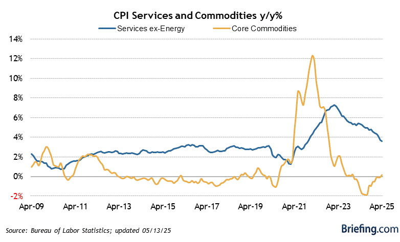 Several market commentators are still worried about the possibility of inflation despite the fact that RMB is most decreasing. This is mostly due to a long-run bull run in commodities driven by agriculture and energy prices and a weaker dollar. Indeed, if we are entering a recession, industrial minerals should be beat down further than they are.
Above are the graphs for the past two years worth of DBA and DBB (the agricultural and base minerals etfs, respectively). DBA (and GLD and USO) have all been on a run lately. Some of this run is certainly based on fundamental factors (ethanol, the collapse of the financial markets, and market's determined belief in peak oil). However, I would caution anyone looking to put on new positions in these commodity classes to hedge your risk by shorting a value of DBB equal to the whole value of those positions. If the market thinks inflation will be coming down, industrial minerals will decline faster than the others since it fundamentally should do that. The spread will certainly widen though it might make sense to wait to put on the long side of the spread until there is a pullback or a naked position on the short side until the recent trend shows signs of ending. You don't have to think that inflation is going to decrease (which it usually does in recessions, but not always), but just that industrial minerals will decrease more than the rest of commodities.
Subscribe to:
Posts (Atom)